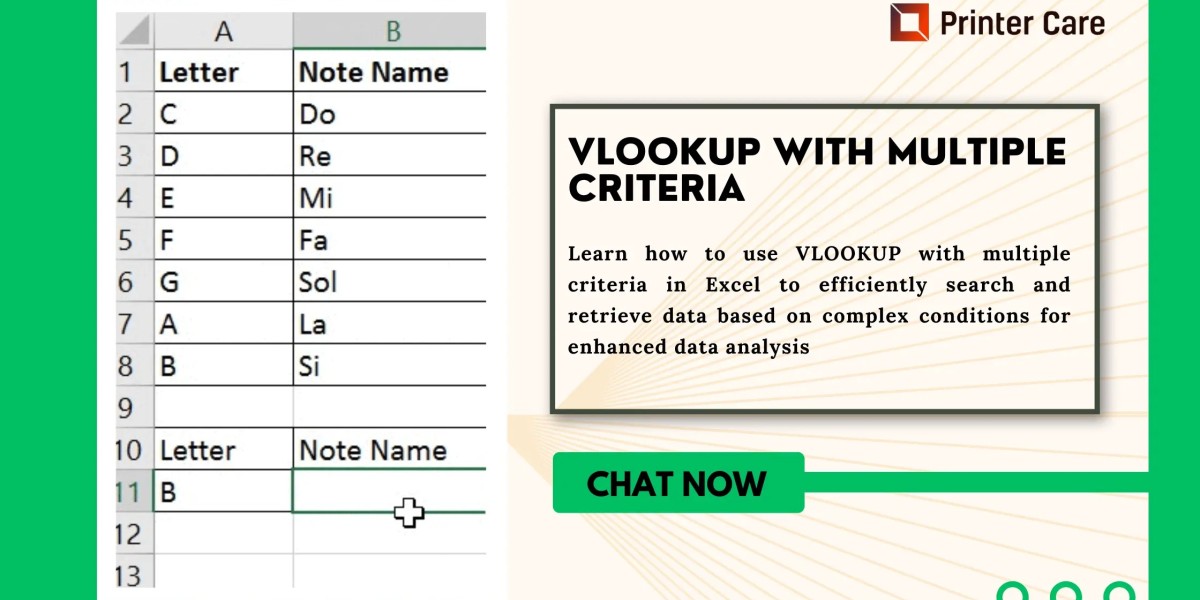
VLOOKUP is one of the most popular Excel functions, helping users retrieve data based on a specific value. However, by default, VLOOKUP only works with a single criterion. So, what if you need to look up data based on multiple conditions? This guide will show you how to use VLOOKUP with multiple criteria efficiently.

Chat with live technician- Click Here

Why Use VLOOKUP with Multiple Criteria?

In many real-world scenarios, you may need to retrieve data based on two or more conditions. For example:

• Looking up an employee’s department and role together.
• Finding product prices based on category and size.
• Searching for student grades based on name and subject.

Since VLOOKUP doesn’t natively support multiple criteria, you need alternative approaches to achieve the desired result.

Method 1: Using a Helper Column

The easiest way to use VLOOKUP with multiple criteria is by combining the criteria into a single helper column.

Steps to Use a Helper Column:

1. Insert a new column at the beginning of your dataset.
2. In this column, combine the values of multiple criteria using the & operator. Example:
   excel Copy

   =A2&B2
   This merges values from Column A (e.g., Employee Name) and Column B (e.g., Department).
3. Use VLOOKUP to search for this combined value:
   excel

   Copy

   =VLOOKUP(D2&E2, A:B, 2, FALSE)
   Here, D2 and E2 contain the lookup values, and A:B is the lookup range.

✅ Pros: Simple and works efficiently.
❌ Cons: Requires modifying the dataset by adding a helper column.

Method 2: Using an Array Formula (for Advanced Users)

If you prefer not to use a helper column, you can use an array formula with INDEX and MATCH.

Steps to Use an Array Formula:

1. Use the following formula to retrieve data based on two criteria:

   excel

   Copy

   =INDEX(C2:C10, MATCH(1, (A2:A10=D2) * (B2:B10=E2), 0))
   • A2:A10 = First criteria column
   • B2:B10 = Second criteria column
   • D2 & E2 = Lookup values
   • C2:C10 = Result column

2. Press Ctrl + Shift + Enter (for Excel 2019 and older) to activate the array formula.

✅ Pros: No need for a helper column.
❌ Cons: More complex and requires understanding of array formulas.

Method 3: Using XLOOKUP (For Newer Excel Versions)

If you’re using Excel 365 or Excel 2019, the XLOOKUP function makes it easier to perform lookups with multiple criteria.

Here’s an example:

This formula searches for rows where both criteria match and returns the corresponding value.

✅ Pros: No helper column needed, easier than array formulas.
❌ Cons: Only available in Excel 365 and later.

Conclusion

Using VLOOKUP with multiple criteria can be tricky, but with the right techniques, you can efficiently search and retrieve data. If you can modify your dataset, a helper column is the easiest method. For advanced users, array formulas and XLOOKUP provide powerful alternatives.